Gravity Model for Park Visitation Inferences

A hybrid spatio-temporal model for hourly park visitation estimation in geographically-distributed parks and public spaces by leveraging multi-source data and confidence weighting
Abstract
Accurate, fine-grained visitation data is crucial for park management, urban planning, and resource allocation. Traditional methods, such as manual counting or permanent sensor installation, are often costly and geographically limited. This study presents a hybrid spatio-temporal modeling framework designed to infer hourly visitation counts for a large portfolio of parks and public spaces. The model integrates a generalized gravity-like approach with machine learning and time-series components to leverage a rich, multi-source dataset. Key inputs include park attributes (amenities, area), population demographics, hourly weather data, and visitation counts from both high-confidence ground truth sensors and lower-confidence crowdsourced mobile data. The model is calibrated using a weighted regression approach, which allows it to learn robust patterns from the more reliable data while incorporating the broader spatiotemporal coverage of the crowdsourced data. The methodology provides a detailed, hourly visitation profile for all parks, even those with no direct monitoring, and demonstrates how a diverse set of inputs can be combined to overcome data limitations and produce actionable insights. A sample dataset and a step-by-step walkthrough are provided to illustrate the practical application of this framework.
Keywords: Spatial Interaction, Gravity Model, Visitation Estimation, Human Mobility, Time Series, Machine Learning, Data Fusion.
1. Introduction
Public parks, trails, lakes, and open spaces serve as vital community assets, offering numerous benefits for physical health, mental well-being, and social cohesion. Effective management and planning of these recreational areas necessitate precise and timely data on visitor dynamics. Understanding when, where, and why people visit these spaces is paramount for optimizing resource allocation, scheduling maintenance, planning events, and ensuring equitable access.
Historically, park visitation data has been collected through labor-intensive manual counting, limited-scope surveys, or fixed-point sensors (e.g., trail counters, infrared sensors, pneumatic tube counters, and traffic cameras). While these methods provide high-confidence "ground truth" data, they are often expensive, geographically sparse, and lack the temporal granularity (e.g., hourly) required for dynamic operational decisions.
The advent of "big data" from mobile devices and crowdsourced applications offers a seemingly abundant alternative for estimating human mobility and visitation. However, such data, derived from a sample of mobile phone users, presents significant challenges:
- Representativeness: The sample of mobile app users may not accurately reflect the entire population of park visitors, leading to biases.
- Accuracy/Confidence: Raw crowdsourced visitation estimates often lack direct validation and can have varying levels of confidence.
- Scaling: Extrapolating from a sample to total visitation requires robust scaling methodologies.
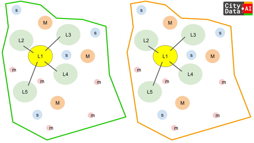
Traditional spatial interaction models, such as the gravity model, provide a foundational framework for understanding movement patterns based on "mass" (attractiveness/population) and "distance" (impedance). While intuitive, basic gravity models often fall short in capturing the intricate spatio-temporal dynamics and heterogeneous influences on modern human mobility, especially at fine temporal granularities (e.g., hourly).
This write-up proposes a novel modeling framework that synthesizes these disparate data sources into a cohesive and robust predictive tool. Our approach builds on the foundational principles of the gravity model, a spatial interaction framework that has been successfully applied to human migration, trade flows, and travel demand. The classic gravity model posits that the flow of people between an origin and a destination is directly proportional to the "masses" of the two locations and inversely proportional to the "distance" between them.
The model presented here extends this simple concept by incorporating a richer set of variables and employing a machine learning methodology. We move beyond a simple product-division form to a more flexible, feature-rich regression-based approach that can learn complex, non-linear relationships. The proposed model is customized to utilize the specific data inputs at our disposal, including detailed park amenities, local demographics, and real-time weather, to produce granular, hourly visitation estimates across a large network of places like 1000 parks, trails, and lakes, even those with no ground truth data.
2. Literature Review (Brief)
Spatial interaction models, rooted in Newton's law of universal gravitation, have long been employed in geography, economics, and transportation planning to predict flows between locations. The foundational gravity model posits that interaction between two places is directly proportional to their "masses" (e.g., populations, economic sizes) and inversely proportional to the square of the distance between them. While simple and intuitive, these models often lack the nuance to capture complex behavioral patterns, competitive effects, and temporal variations. See References.
Subsequent developments introduced constrained gravity models (e.g., production-constrained, attraction-constrained, doubly-constrained) to ensure consistency with known origin or destination totals. Destination choice models, a more behaviorally explicit alternative, model the probability of an individual selecting a destination from a set of alternatives based on attributes of the traveler and the destinations.
The proliferation of digital data sources, including geolocated social media, mobile phone data, and web search queries, has revolutionized human mobility research. These "big data" sources offer unprecedented spatial and temporal granularity, enabling real-time monitoring and prediction of human movement. However, the inherent biases, sampling issues, and varying confidence levels in crowdsourced data necessitate advanced methodologies for accurate inference.
Machine learning (ML) techniques, such as Artificial Neural Networks (ANNs), Support Vector Machines (SVMs), Random Forests, and Gradient Boosting models, have demonstrated superior predictive capabilities in complex, non-linear systems, making them highly suitable for tourism and mobility forecasting. The challenge lies in effectively integrating these diverse data sources and modeling paradigms to produce reliable, granular visitation estimates. This paper aims to bridge this gap by proposing a hybrid approach that leverages the strengths of gravity-like principles, rich spatio-temporal features, and weighted machine learning.
3. Data Inputs
The proposed model is designed to utilize the following comprehensive dataset:
- Place/Geofence Data:
Place Name: Unique identifier for each park/geofence.Category: Categorical classification (e.g., "Park," "Trail," "Lake," "Open Space," "Fishery," "Campground").GeoJSON Shape: Exact polygonal boundary for each geofence.Area: Calculated area in square meters for each geofence.Centroid: Latitude and longitude coordinates for distance calculations.
- Amenity Data (per park):
- Detailed list of amenities: restrooms, play areas, BBQ grills, picnic tables, tennis courts, baseball fields, basketball courts, pickleball courts, volleyball courts, grassy lawns, drinking fountains, splash pads, etc. (Binary presence/absence or counts).
- Surrounding Place Data (per park):
- List of nearby points of interest (POIs) within a defined radius (e.g., 1km, 5km): retail locations, coffee shops, pharmacies, restaurants, malls, community centers, emergency services, clinics, hospitals. (Counts or aggregated measures).
- Population & Demographics (US Census & ACS data):
Neighborhood Census Block Level: Population counts and detailed demographic characteristics (e.g., median income, age distribution, household size, vehicle ownership, presence of children) for all relevant origin census blocks.
- Weather Time Series Data:
- Hourly data for relevant weather stations, including:
temperature,rainfall,snowfall,humidity,visibility.
- Hourly data for relevant weather stations, including:
- Visitation Counts (Target Variable Data):
- High-Confidence Data (30% of parks): Monthly counts from actual manual counting surveys and IoT sensors. This serves as ground truth.
- Low-Confidence Data (70% of parks): Hourly estimates derived from crowdsourced mobile apps. These require careful scaling and confidence weighting.
4. Methodology
Our approach is a multi-stage, data-driven methodology that combines feature engineering, weighted regression, and a spatio-temporal modeling strategy.
4.1. Data Preprocessing and Feature Engineering
The quality of the model's output is highly dependent on the quality and richness of its input features. We transform the raw data into a structured dataset for model training.
A. Spatial Features (Gravity Model Components):
The core of our model is the relationship between potential visitor origins and park destinations.
- Destinations (Aj): Each of the 1,000 geofences is treated as a destination j. We create a feature vector for each destination, including:
Area_j: Area in square meters from GeoJSON.Category_j: One-hot encoded category (e.g., Park, Trail, Lake).Amenities_j: A series of binary (0/1) features for the presence of each amenity (e.g., restrooms, play areas, splash pads).Context_j: Features capturing the number of nearby amenities (e.g.,num_restaurants_1km,has_pharmacy_500m).
- Origins (Pi): US Census Block Groups serve as our origins i. We use their total population and key demographic variables (e.g., median household income, children per household).
- Distance/Impedance (Dij): We calculate road travel time (in minutes) between the centroid of each origin i and each destination j. A distance matrix is pre-computed and stored for efficiency.
- Gravity-based Features: Instead of a single gravity formula, we create aggregated features that encapsulate the gravity concept for a given park j. For each park, we compute a weighted sum of populations in its catchment area:
- \[ \text{PopProximity}_j = \sum_{i \in \text{catchment}} \frac{P_i^\alpha}{D_{ij}^\gamma} \]
- The parameters α and γ will be learned implicitly by the model, but we can simplify by using a standard inverse-square distance decay initially (γ=2). A more advanced approach would be to create several such features with varying γ values (e.g., γ=1,2,3) and let the model determine their importance.
B. Temporal Features:
We create features to capture hourly, daily, and seasonal patterns:
Hour_h: An hour of day (0-23) feature, often transformed using sine and cosine functions to capture its cyclical nature:- \[ \text{hour\_sin} = \sin(2 \pi \cdot \text{hour} / 24) \]
- \[ \text{hour\_cos} = \cos(2 \pi \cdot \text{hour} / 24) \]
Day_of_Week: One-hot encoded (Monday-Sunday).Weekend_Flag,Holiday_Flag,School_Holiday_Flag: Binary flags.Month_morDay_of_Year: Cyclical features to capture seasonal trends.
C. Environmental Features:
Hourly weather data is aligned with each park's visitation data.
Temperature_h,Rainfall_h,Snowfall_h,Humidity_h,Visibility_h.- We also include lagged features (e.g.,
Rainfall_h-1,Temperature_avg_24h) and interaction features (e.g.,Temp_h×HasSplashPad_j) to capture more complex relationships.
D. Visitation Data Scaling and Confidence Weighting:
This is a crucial step to handle the discrepancy in data quality.
- Ground Truth Data: For the 30% of parks with manual/IoT data, their hourly counts are our high-confidence target variable. Each observation is assigned a confidence weight of Wtrue=1.0.
- Crowdsourced Data: For the remaining 70% of parks, the hourly crowdsourced estimates are used, but they are first scaled to approximate total visitation. We derive a scaling factor for each park or category of park by comparing the ground truth data to the crowdsourced data for the 30% of parks where both exist. The confidence weight for each crowdsourced observation, Wcrowd, is set to a value between 0 and 1, based on the statistical confidence in the crowdsourced estimate itself (e.g., a function of the sample size of mobile devices).
4.2. Model Selection and Training
We utilize a supervised learning approach, specifically a weighted ensemble tree model such as a Gradient Boosting Regressor (e.g., XGBoost or LightGBM). This choice is motivated by its ability to handle non-linear relationships, interaction effects between features, and a large number of predictors, all while naturally supporting a sample_weight parameter for our confidence weights.
The training dataset consists of hourly observations for all 1000 parks over a defined period. The target variable is the hourly visitation count, Vj,h.
The model's objective is to minimize a loss function (e.g., Mean Squared Error or a Poisson loss function appropriate for count data) weighted by the confidence score:
\[ \text{Loss} = \sum_{j,h} W_{j,h} \cdot \mathcal{L}(V_{j,h}, \hat{V}_{j,h}) \]
Where:
- Wj,h: The confidence weight for the observation at park j and hour h.
- L(⋅,⋅): The loss function.
- V^j,h: The model's predicted visitation count.
The trained model effectively learns the complex function:
\[ \hat{V}_{j,h} = f(\text{Features}_j, \text{Features}_{i \rightarrow j}, \text{Features}_{h,d,m}, \text{Features}_{weather}) \]
4.3. Hourly Visitation Inference
After calibration, the model can be used to predict hourly visitation for all 1000 parks for any desired time period. For the parks without ground truth, we simply input their unique feature set (amenities, area, etc.) along with the corresponding hourly temporal and weather data. The model uses the relationships it learned from the 30% high-confidence data and the 70% weighted crowdsourced data to make robust predictions. The model can even predict visitation for new parks (not in the original dataset) as long as their features are provided.
5. Conclusion
Accurate hourly visitation counts are indispensable for the effective management of recreational spaces. This paper outlines a robust hybrid spatio-temporal modeling approach that extends the traditional gravity model to meet this demand, particularly in data-rich but confidence-variable environments. By meticulously engineering features from diverse data sources (geofences, amenities, demographics, weather, and surrounding POIs) and employing a weighted machine learning regression framework, the proposed model can:
- Integrate Heterogeneous Data: Effectively combine high-confidence ground truth data with lower-confidence crowdsourced mobile app data.
- Capture Complex Dynamics: Account for spatial accessibility (gravity component), temporal patterns (hourly, daily, seasonal), and environmental influences (weather).
- Provide Granular Estimates: Output hourly visitation counts across all parks, enabling dynamic operational decisions.
- Leverage Confidence: Prioritize reliable data during model training through explicit weighting.
While the implementation requires significant data engineering and computational resources, the resulting accurate and granular visitation profiles offer unparalleled insights for park managers, urban planners, and policymakers. This methodology provides a scalable and adaptable solution for understanding and optimizing human interaction with vital public recreational assets. Future work could explore the integration of real-time event data, public transport accessibility, and more advanced deep learning architectures for further predictive enhancements.
6. References
Zipf, G. K. (1946). The P1 P2/D Hypothesis: On the Intercity Movement of Persons. American Sociological Review, 11(6), 676-686.
Wilson, A. G. (1971). A family of spatial interaction models, and associated developments. Environment and Planning A, 3(1), 1-32.
McFadden, D. (1974). Conditional Logit Analysis of Qualitative Choice Behavior. In P. Zarembka (Ed.), Frontiers in Econometrics (pp. 105-142). Academic Press.
Cici, S., & Basso, A. (2020). Human mobility analysis from big data: A review. Journal of Big Data, 7(1), 1-28.
Wood, S. A., Guerry, A. D., Silver, J. M., & Lacayo, M. (2013). Using social media to quantify nature-based recreation: A case study from the San Francisco Bay Area. Journal of Environmental Management, 131, 150-157.
Tenkanen, H., Di Minin, E., Heikinheimo, V., Hausmann, A., Herder, N. L., & Toivonen, T. (2017). Instagram data reveal patterns of nature-based recreation across Europe. Applied Geography, 89, 13-22.
Song, H., & Li, G. (2008). A review of tourism demand modeling and forecasting: The past, the present and the future. Tourism Management, 29(2), 203-220.
Sun, S., & Law, R. (2019). The application of machine learning in tourism and hospitality research: A review. Journal of Hospitality & Tourism Research, 43(1), 3-23.
7. Sample Dataset and Step-by-Step Walkthrough
Based on the detailed methodology provided, the model's predicted visitation count formula is best represented in a generalized linear model (GLM) form, which is then handled by a machine learning framework.
\[ \lambda_{j,h,d,m,y} = \exp(\beta_0 + \sum \beta_P \cdot \ln(P_i) - \sum \beta_D \cdot \ln(D_{ij}) \\ + \sum \beta_A \cdot \text{Amenity\_Features}_j \\ + \sum \beta_S \cdot \text{Surrounding\_Places}_j \\ + \sum \beta_T \cdot \text{Temporal\_Features}_{h,d,m,y} \\ + \sum \beta_W \cdot \text{Weather\_Features}_{h,d,m,y} \\ + \sum \beta_{\text{Int}} \cdot \text{Interactions}) \]
To demonstrate the process, we'll create a simplified dataset with 20 parks over a single day, with hourly data from 9 AM to 5 PM.
7.1. Sample Data Inputs
A. Park Geofence & Amenities Data (20 parks total)
| Park ID | Park Name | Category | Area (m²) | HasRestrooms | HasPlayArea | HasSplashPad | Surrounding_Score | GroundTruth |
| P1 | Park A | Park | 5000 | 1 | 1 | 0 | 0.8 | YES |
| P2 | Park B | Park | 8500 | 1 | 1 | 1 | 0.9 | YES |
| P3 | Park C | Trail | 20000 | 0 | 0 | 0 | 0.5 | NO |
| P4 | Park D | Park | 6000 | 1 | 0 | 0 | 0.6 | YES |
| P5 | Park E | Open Space | 15000 | 0 | 0 | 0 | 0.4 | NO |
| P6 | Park F | Park | 9500 | 1 | 1 | 0 | 0.85 | YES |
| P7 | Park G | Lake | 50000 | 1 | 1 | 0 | 0.7 | NO |
| P8 | Park H | Park | 4500 | 0 | 1 | 0 | 0.9 | NO |
| P9 | Park I | Park | 7000 | 1 | 0 | 0 | 0.75 | YES |
| P10 | Park J | Trail | 18000 | 0 | 0 | 0 | 0.6 | NO |
| P11 | Park K | Lake | 60000 | 1 | 0 | 0 | 0.5 | YES |
| P12 | Park L | Park | 12000 | 1 | 1 | 1 | 0.8 | NO |
| P13 | Park M | Trail | 25000 | 0 | 0 | 0 | 0.45 | NO |
| P14 | Park N | Park | 7500 | 1 | 1 | 0 | 0.9 | NO |
| P15 | Park O | Park | 5500 | 1 | 0 | 0 | 0.65 | NO |
| P16 | Park P | Park | 10000 | 1 | 1 | 0 | 0.7 | NO |
| P17 | Park Q | Trail | 14000 | 0 | 0 | 0 | 0.3 | NO |
| P18 | Park R | Park | 8000 | 1 | 1 | 1 | 0.75 | NO |
| P19 | Park S | Lake | 45000 | 1 | 1 | 0 | 0.6 | NO |
| P20 | Park T | Park | 11000 | 1 | 0 | 0 | 0.85 | NO |
B. Census/Population Data (Simplified):
Assume 10 nearby census block groups with varying populations and distances to each park. From this, we calculate a single PopProximity score for each park.
| Park ID | PopProximity |
| P1 | 1500 |
| P2 | 2500 |
| P3 | 800 |
| ... | ... |
| P20 | 1800 |
C. Hourly Data (Temperature, Visitation):
Assume a single day (e.g., Saturday) with hourly data for a specific hour (e.g., 2 PM).
| Hour | Day_of_Week | Temp (°C) | Rainfall (mm) | Weekend_Flag |
| 14 | Saturday | 25 | 0 | 1 |
D. Visitation Data by Park and Hour:
- Ground Truth (6 parks): | Park ID | Hour | Vis. Count (Manual) | Source_Confidence | |:—:|:—:|:—:|:—:| | P1 | 14 | 120 | 1.0 | | P2 | 14 | 250 | 1.0 | | P4 | 14 | 80 | 1.0 | | P6 | 14 | 150 | 1.0 | | P9 | 14 | 100 | 1.0 | | P11| 14 | 200 | 1.0 |
- Crowdsourced (All 20 parks): | Park ID | Hour | Vis. Count (Crowdsourced) | Confidence_Weight | |:—:|:—:|:—:|:—:| | P1 | 14 | 100 | 0.8 | | P2 | 14 | 220 | 0.8 | | P3 | 14 | 30 | 0.6 | | P4 | 14 | 75 | 0.8 | | ... | ... | ... | ... | | P18 | 14 | 180 | 0.7 |
7.2. Step-by-Step Walkthrough to Infer Visitation
Step 1: Data Preprocessing and Feature Engineering
We combine all our inputs into a single training dataset. For a single observation (2 PM on a Saturday at Park B), a row would look like this:
| Feature | Value |
Park_ID | P2 |
Area | 8500 |
IsPark | 1 |
IsTrail | 0 |
HasRestrooms | 1 |
HasPlayArea | 1 |
HasSplashPad | 1 |
Surrounding_Score | 0.9 |
PopProximity | 2500 |
Hour | 14 |
Temp | 25 |
Rainfall | 0 |
Weekend_Flag | 1 |
Vis_Count | 250 |
Confidence_Weight | 1.0 |
Step 2: Model Calibration
We train a regression model (e.g., XGBoost) on this combined dataset. The model learns the complex relationships between all the input features and the Vis_Count, while giving more importance to the data rows with a Confidence_Weight of 1.0.
For example, the model would learn:
HasSplashPadis a very strong predictor of visitation on a hot day (Temp> 20°C).PopProximityis a fundamental driver of a park's overall visitation level.- The
IsTrailcategory correlates with lower total visitation but a more consistent hourly flow during the day. - The
Surrounding_Scorehas a positive but smaller effect on visitation.
Step 3: Inference for Parks without Ground Truth
Now, we use our trained model to predict visitation for the 14 parks (e.g., P3, P5, P7) that only have crowdsourced data. We simply feed the model their specific features, along with the hourly temporal and weather data.
For Park P3 (a trail with low PopProximity and no amenities), the input might be: {Area: 20000, IsPark: 0, IsTrail: 1, HasRestrooms: 0, HasPlayArea: 0, HasSplashPad: 0, PopProximity: 800, Hour: 14, Temp: 25, Rainfall: 0, Weekend_Flag: 1, Surrounding_Score: 0.5}
The model, based on its learned parameters, would combine these inputs to output a predicted visitation count. It would see that the park is large but has low PopProximity and no amenities, which would lead to a lower-than-average prediction. However, as it is a trail, it might predict a more consistent, lower flow of visitors compared to a playground park.
For Park P18 (a park with amenities and a high Surrounding_Score), the input might be: {Area: 8000, IsPark: 1, IsTrail: 0, HasRestrooms: 1, HasPlayArea: 1, HasSplashPad: 1, PopProximity: 2000, Hour: 14, Temp: 25, Rainfall: 0, Weekend_Flag: 1, Surrounding_Score: 0.75}
The model would identify the presence of a HasSplashPad on a hot day (Temp > 20°C), and a good PopProximity and Surrounding_Score, which would likely result in a high predicted visitation count.
The model is able to make these inferences because it was trained on the rich patterns found in the ground truth data and the broader spatial and temporal coverage of the crowdsourced data. The confidence weights ensure that the model doesn't overfit to the noise in the crowdsourced data while still learning from its valuable scale. The final output is an hourly visitation estimate for all 20 parks, providing comprehensive insights for park management.
About CITYDATA.ai
CITYDATA.ai provides mobility big data + AI to make cities smarter, sustainable, and more resilient. We provide insights about people counts, density patterns, movement trends, economic impact, and community engagement.
Founded in 2020 in San Francisco, California, CITYDATA.ai provides fresh, accurate, daily insights that are essential for smart city programs, economic development, urban planning, mobility and transportation, tourism, parks and recreation, disaster mitigation, sustainability, and resilience.
You can reach us via email at business@citydata.ai if you’d like to discuss your data needs and use cases. You can also follow the company on Linkedin, and subscribe to our blog to stay updated on the newest innovations in big data and AI for the public sector.